Probabilistic modeling

Problem statement

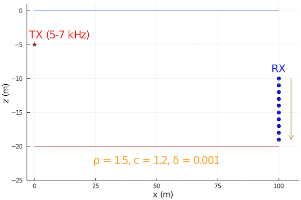
Let us consider a geoacoustic inversion problem where we have a static omnidirectional broadband acoustic source transmitting in a 5-7 kHz band. A single omnidirectional receiver picks up the signal at a fixed range, but profiles the water column, and therefore makes transmission loss measurements at various depths. We would like to estimate seabed parameters from these transmission loss measurements.

Dataset

To illustrate this idea, let us generate a synthetic dataset for a known set of seabed parameters (relative density ρ = 1.5, relative soundspeed c = 1.2, and attenuation δ = 0.001).

The environment is assumed to be an isovelocity and with a constant depth of 20 m. The source is at a depth of 5 m. The receiver is at a range of 100 m from the source, and makes measurements at depths from 10 to 19 m in steps of 1 m.

Since we have an range-independent isovelocity environment, we can use the PekerisRayModel (otherwise we could use the RaySolver):

using UnderwaterAcoustics
using DataFrames

function 𝒴(θ)
  r, d, f, ρ, c, δ = θ
  env = UnderwaterEnvironment(seabed = RayleighReflectionCoef(ρ, c, δ))
  tx = AcousticSource(0.0, -5.0, f)
  rx = AcousticReceiver(r, -d)
  pm = PekerisRayModel(env, 7)
  transmissionloss(pm, tx, rx)
end

data = [
  (depth=d, frequency=f, xloss=𝒴([100.0, d, f, 1.5, 1.2, 0.001]))
  for d ∈ 10.0:1.0:19.0, f ∈ 5000.0:100.0:7000.0
]
data = DataFrame(vec(data))

Probabilistic model

We use some very loose uniform priors for ρ, c and δ, and estimate the transmission loss using the same model 𝒴, as used in the data generation, but without information on the actual seabed parameters. We assume that the measurements of transmission loss are normally distributed around the modeled transmission loss, with a covariance of 0.5 dB.

We define the probabilistic model as a Turing.jl model:

using Turing

# depths d, frequencies f, transmission loss measurements x
@model function geoacoustic(d, f, x)
  ρ ~ Uniform(1.0, 3.0)
  c ~ Uniform(0.5, 2.5)
  δ ~ Uniform(0.0, 0.003)
  μ = [𝒴([100.0, d[i], f[i], ρ, c, δ]) for i ∈ 1:length(d)]
  x ~ MvNormal(μ, 0.5)
end

Variational inference

Once we have the model defined, we can run Bayesian inference on it. We could either use MCMC methods from Turing, or variational inference. Since our model is differentiable, we choose to use the automatic differentiation variational inference (ADVI):

using Turing: Variational

q = vi(
  geoacoustic(data.depth, data.frequency, data.xloss),
  ADVI(100, 10000)
)

The returned q is a 3-dimensional posterior probability distribution over the parameters ρ, c and δ. We can estimate the mean of the distribution by drawing random variates and taking the sample mean:

julia> mean(rand(q, 10000); dims=2)
3×1 Array{Float64,2}:
 1.4989510476936188
 1.2000012848664092
 0.0009835578241605488

We see that the estimated parameter means for ρ, c and δ are quite close to the actual values used in generating the data.

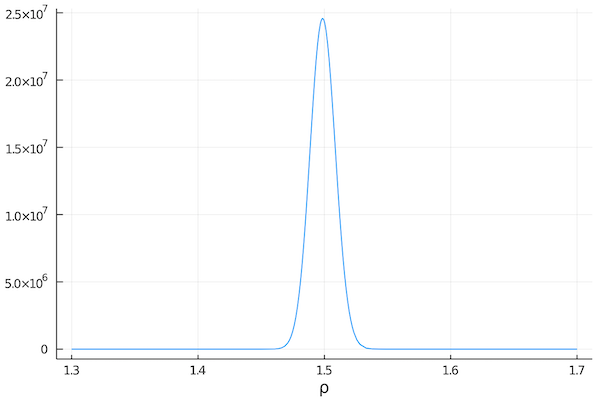
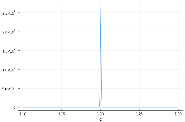
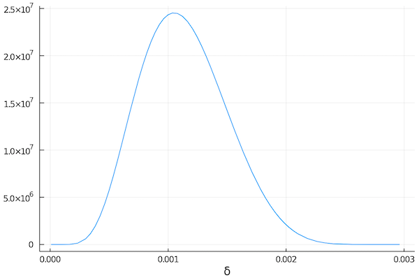
We can also plot the conditional distributions of each parameter:

using StatsPlots

plot(ρ -> pdf(q, [ρ, 1.2, 0.001]), 1.3, 1.7; xlabel="ρ")
plot(c -> pdf(q, [1.5, c, 0.001]), 1.1, 1.3; xlabel="c")
plot(δ -> pdf(q, [1.5, 1.2, δ]), 0.0, 0.003; xlabel="δ")