Calling from Python

Installation

While UnderwaterAcoustics.jl is written in Julia, it can be called from Python using JuliaCall. For this, we need to install the juliacall package. For some of the examples below, we will also need to numpy and matplotlib, so let’s install them as well:

pip install juliacall numpy matplotlib

Next, we will need to install UnderwaterAcoustics.jl and optionally Plots.jl. To do this, start a Python interpreter and run the following commands:

import juliapkg
juliapkg.add("UnderwaterAcoustics", "0efb1f7a-1ce7-46d2-9f48-546a4c8fbb99")
juliapkg.add("Plots", "91a5bcdd-55d7-5caf-9e0b-520d859cae80")

Tip

While Plots.jl is not necessary if you plan to use matplotlib for plotting, we install it here to demonstrate its use from Python. The plot recipes for Plots.jl that come with UnderwaterAcoustics.jl are very convenient and work nicely if you using Plots.jl from Python. If you use matplotlib, you will need to write your own plotting code based on the data returned from UnderwaterAcoustics.jl. We will show examples of both approaches below.

Getting started

Now we are ready to use UnderwaterAcoustics.jl from Python. To load the package from Python:

from juliacall import Main as jl
jl.seval("using UnderwaterAcoustics")

Let’s start with a simple example similar to the one shown in Quickstart:

env = jl.UnderwaterEnvironment(bathymetry=20, seabed=jl.SandyClay)
pm = jl.PekerisRayTracer(env)
tx = jl.AcousticSource(0.0, -5.0, 1000.0)
rx = jl.AcousticReceiver(100.0, -10.0)
rays = jl.arrivals(pm, tx, rx)

We can display the ray arrivals:

rays

7 element Vector{RayArrival}:
∠ -2.9°  0⤒  0⤓ ∠  2.9° |  65.06 ms | -40.0 dB ϕ   0.0°↝
∠  8.5°  1⤒  0⤓ ∠  8.5° |  65.71 ms | -40.1 dB ϕ 180.0°↝
∠-14.0°  0⤒  1⤓ ∠-14.0° |  66.98 ms | -62.6 dB ϕ 170.9°↝
∠ 19.3°  1⤒  1⤓ ∠-19.3° |  68.85 ms | -74.3 dB ϕ -23.4°↝
∠-24.2°  1⤒  1⤓ ∠ 24.2° |  71.26 ms | -80.4 dB ϕ-145.6°↝
∠ 28.8°  2⤒  1⤓ ∠ 28.8° |  74.16 ms | -73.5 dB ϕ  10.8°↝
∠-33.0°  1⤒  2⤓ ∠-33.0° |  77.50 ms | -100.7 dB ϕ-167.2°↝

or plot them using Plots.jl:

jl.seval("using Plots")               # python doesn't support "!", so we create
jl.seval("plot_add = plot!")          #  an alias plot_add for plot! in Julia

p = jl.plot(env, xlims=(-10,110))
jl.plot_add(tx)
jl.plot_add(rx)
jl.plot_add(rays)
jl.display(p)

We can also get the acoustic field or the transmission loss:

jl.acoustic_field(pm, tx, rx)

0.011324695913076596 + 0.013441491695419415im

jl.transmission_loss(pm, tx, rx)

35.10150548468688

We can also create a grid of receivers and compute the acoustic field over the grid:

rxs = jl.AcousticReceiverGrid2D(jl.range(1.0, 100, step=0.1), jl.range(-20, 0, step=0.1))
x = jl.transmission_loss(pm, tx, rxs)

We can display the transmission loss grid or plot it using Plots.jl:

991×201 Matrix{Float64}:
 19.1283  19.2328  19.5428  19.8492  …   8.82646  11.1099  16.4209  87.1226
 19.1329  19.2373  19.5471  19.8536      8.87496  11.1689  16.4855  87.1228
 19.1381  19.2424  19.552   19.8586      8.92702  11.2323  16.5549  87.1232
 19.1441  19.2483  19.5577  19.8643      8.9824   11.2997  16.6288  87.1235
 19.151   19.255   19.5641  19.8709      9.04085  11.3708  16.7068  87.1239
 19.1587  19.2626  19.5715  19.8784  …   9.10213  11.4454  16.7886  87.1243
 19.1674  19.2712  19.5799  19.8869      9.16605  11.5232  16.8739  87.1247
 19.1772  19.2809  19.5893  19.8965      9.23241  11.604   16.9625  87.1251
 19.1882  19.2918  19.6     19.9073      9.30109  11.6875  17.0541  87.1256
 19.2005  19.3039  19.6119  19.9194      9.37202  11.7737  17.1485  87.1261
  ⋮                                  ⋱                               ⋮
 37.3743  37.4386  37.4768  37.492      57.8842   61.3577  67.2494  98.1616
 37.4077  37.474   37.5142  37.5316     57.9055   61.3787  67.2687  98.1828
 37.442   37.5103  37.5526  37.5721     57.9268   61.4     67.2892  98.2041
 37.4772  37.5475  37.5919  37.6135  …  57.948    61.4216  67.3108  98.2254
 37.5133  37.5856  37.632   37.6557     57.9692   61.4434  67.3335  98.2468
 37.5502  37.6246  37.673   37.6988     57.9903   61.4655  67.3572  98.2682
 37.5881  37.6644  37.7149  37.7427     58.0112   61.4876  67.3819  98.2895
 37.6268  37.7052  37.7577  37.7875     58.0319   61.5099  67.4075  98.311
 37.6664  37.7468  37.8013  37.8331  …  58.0524   61.5322  67.4338  98.3324

p = jl.plot(env, xlims=(0,100))
jl.plot_add(rxs, x)
jl.display(p)

Plotting with `matplotlib`

If you prefer to use matplotlib for plotting, you can use the data returned from UnderwaterAcoustics.jl to create your own plots:

import numpy as np
import matplotlib.pyplot as plt

xloss = np.flipud(np.array(x).transpose())
nz, nx = xloss.shape
x_axis = np.linspace(0, 100, nx)
z_axis = np.linspace(0, -20, nz)
plt.figure()
mesh = plt.pcolormesh(x_axis, z_axis, xloss, shading='auto', cmap='viridis_r', vmin=0, vmax=42)
cbar = plt.colorbar(mesh)
cbar.set_label('Transmission loss (dB)')
plt.xlabel('x (m)')
plt.ylabel('z (m)')
plt.tight_layout()
plt.show()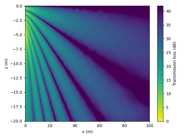

More propagation models

Using other acoustic propagation models such as Bellhop, Kraken, etc is a breeze. During installation, include the relevant Julia packages. For example, to use Bellhop or Kraken, include AcousticToolbox.jl:

import juliapkg
juliapkg.add("AcousticsToolbox", "268a15bc-5756-47d6-9bea-fa5dc21c97f8")

Note

To use models like Bellhop, Kraken, etc, you will NOT need to install the FORTRAN binaries separately. They are automatically installed when you install the relevant Julia packages.

To use the propagation models from AcousticToolbox.jl:

from juliacall import Main as jl
jl.seval("using UnderwaterAcoustics")
jl.seval("using AcousticsToolbox")

bathy = jl.SampledField(np.array([200, 150]), x=np.array([0, 1000]))
ssp = jl.SampledField(np.array([1500, 1480, 1495, 1510, 1520]), z=jl.range(0, -200, step=-50), interp=jl.CubicSpline())
env = jl.UnderwaterEnvironment(bathymetry=bathy, soundspeed=ssp, seabed=jl.SandyClay)
pm = jl.Bellhop(env)
tx = jl.AcousticSource(0.0, -5.0, 1000.0)
rx = jl.AcousticReceiver(100.0, -10.0)
rays = jl.arrivals(pm, tx, rx)

7 element Vector{RayArrival}:
∠ -9.0°  0⤒  0⤓ ∠ -3.8° | 672.12 ms | -60.5 dB ϕ   0.0°↝
∠-13.2°  0⤒  1⤓ ∠-14.3° | 677.43 ms | -88.6 dB ϕ 129.4°↝
∠ 10.3°  1⤒  0⤓ ∠  6.3° | 680.38 ms | -60.3 dB ϕ 180.0°↝
∠ 16.2°  1⤒  1⤓ ∠-18.9° | 693.31 ms | -87.7 dB ϕ-156.5°↝
∠-20.9°  1⤒  1⤓ ∠ 24.4° | 724.26 ms | -87.4 dB ϕ-168.6°↝
∠ 24.9°  2⤒  1⤓ ∠ 29.0° | 749.86 ms | -85.4 dB ϕ   6.1°↝
∠ 35.5°  3⤒  2⤓ ∠ 45.7° | 877.95 ms | -108.0 dB ϕ-175.2°↝

jl.seval("using Plots")
jl.seval("plot_add = plot!")

p = jl.plot(env, xlims=(-10,110))
jl.plot_add(tx)
jl.plot_add(rx)
jl.plot_add(rays)
jl.display(p)

Channel modeling

We can also access the channel modeling API from Python. For example, we can obtain a channel from a propagation model:

env = jl.UnderwaterEnvironment(bathymetry=20, seabed=jl.SandyClay)
pm = jl.PekerisRayTracer(env)
tx = jl.AcousticSource(0.0, -5.0, 1000.0, spl=170)
rx = jl.AcousticReceiver(100.0, -10.0)
fs = 192000
ch = jl.channel(pm, tx, rx, fs, noise=jl.RedGaussianNoise(0.5e6))

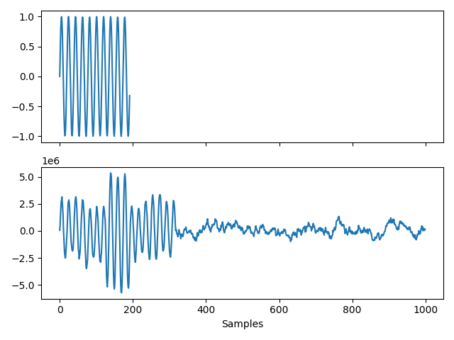
We can then create a signal and pass it through the channel:

import numpy as np

x = np.sin(2 * np.pi * 10000 * np.arange(0, 0.001, 1/fs))
y = jl.transmit(ch, x, fs=fs)  # returned signal is a Julia SampledSignal object
y = np.array(y)                # so we convert it to a numpy array

and plot it using matplotlib:

import matplotlib.pyplot as plt

fig, (ax1, ax2) = plt.subplots(2, 1, sharex=True)
ax1.plot(x)
ax2.plot(y[:1000])
ax2.set_xlabel("Samples")
plt.tight_layout()
plt.show()